Example usage

To see how pysentimentanalyzer works, we will illustrate it with some sample text from disaster tweets.

import pandas as pd
from pysentimentanalyzer.generate_wordcloud import *
from pysentimentanalyzer.get_aggregated_sentiment_score import *
from pysentimentanalyzer.likert_scale import *
from pysentimentanalyzer.sentiment_score_plot import *

df = pd.read_csv("../tests/test_tweets.csv") # assuming the csv exists in the current directory
df = df.head(200)
df.head()

[nltk_data] Downloading package vader_lexicon to
[nltk_data]     /home/docs/nltk_data...
[nltk_data]   Package vader_lexicon is already up-to-date!
[nltk_data] Downloading package punkt to /home/docs/nltk_data...
[nltk_data]   Package punkt is already up-to-date!

	id	keyword	location	text
0	0	ablaze	NaN	Communal violence in Bhainsa, Telangana. "Ston...
1	1	ablaze	NaN	Telangana: Section 144 has been imposed in Bha...
2	2	ablaze	New York City	Arsonist sets cars ablaze at dealership https:...
3	3	ablaze	Morgantown, WV	Arsonist sets cars ablaze at dealership https:...
4	4	ablaze	NaN	"Lord Jesus, your love brings freedom and pard...

We will only be interested in working with the text column.

To get an overall sentiment of the texts in the text column, we can use the function aggregate_sentiment_score to get the average compound score (sentiment).

aggregate_sentiment_score(df, "text")

-0.143

Given that this value is not very interpretable, we can use the function convert_to_likert to get something that makes more sense.

convert_to_likert(df, "text")

('neutral', 3)

This makes a lot more sense. While the average compound score is negative, suggesting that the sentiment is negative, since the value is fairly close to 0, the sentiment is closer to being neutral rather than negative. Thus, on a likert scale, the sentiment is neutral.

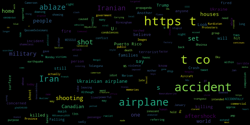
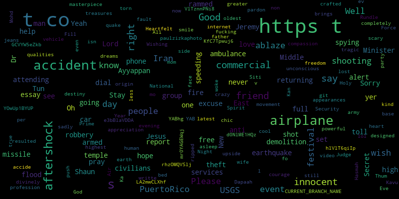
To see what words occur frequently, we can use the generate_wordcloud function. The function returns a list of three values corresponding to:

1. most frequent words from positive texts

2. most frequent words from neutral texts

3. most frequent words from negative texts

wc = generate_wordcloud(df, "text")
wc[0]

wc[1]

wc[2]

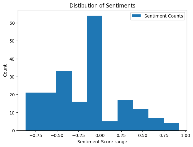
Finally, the function sentiment_score_plot returns a histogram of the compound scores for the texts. This allows us to easily visualize the distribution of the sentiments in all the texts.

plot = sentiment_score_plot(df, "text")
plot

The highest frequency (64.0) of sentiment scores are in range -0.1 to 0.0 which forms 32.00% of samples in the dataset